Having opened an experimental datafile using the Sampling page, you may now decide to input the Channel porosity rather than the Open porosity. As previously stated on the Sampling page, this is the porosity visible from an electron micrograph of the surface, as a channel passing through the sample. It will normally be less than the Open porosity, because if pores within the matrix of the porous material are larger than the throats connecting them to the surface, some or most of their volume will be concealed in a micrograph of the surface.
In the example case of the graphite shown below, the Open porosity is 12.61%, but say we have measured the channel porosity from image analysis of an electron micrograph as 2.67%. Click on the small down-arrow next to Advanced, and scroll down the Advanced sub-screen until you see the relevant details. Enter the value of the channel porosity as shown:
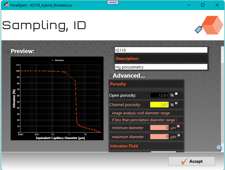
On entering the channel porosity, the image analysis cylindrical equivalent void diameter range entry boxes are displayed, as shown above. To use the default values, i.e. the whole range of sizes, click the check-boxes next to minimum diameter and maximum diameter, and those values will be displayed.
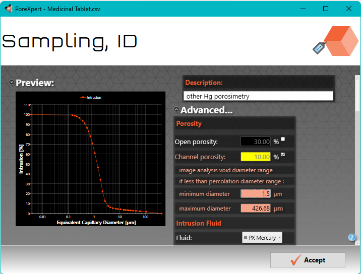
However, it is very often impossible to carry out image analysis over the whole size range. If you have carried out the image analysis over a smaller size range, for example because any voids below 1.12 μm cylindrical-equivalent diameter cannot be distinguished from surface imperfections, then input the channel porosity range as shown below. Note that you do not have to input both limits of the range - if one limit is the same diameter as one of the percolation range limits, then just click the check-box to display the default value. As shown below, as a visual clue, entries associated with channel porosity are shown PoreXpert brown on this and the curve fitting screen.
Having clicked the Accept button, we are taken to the Curve Fitting window.
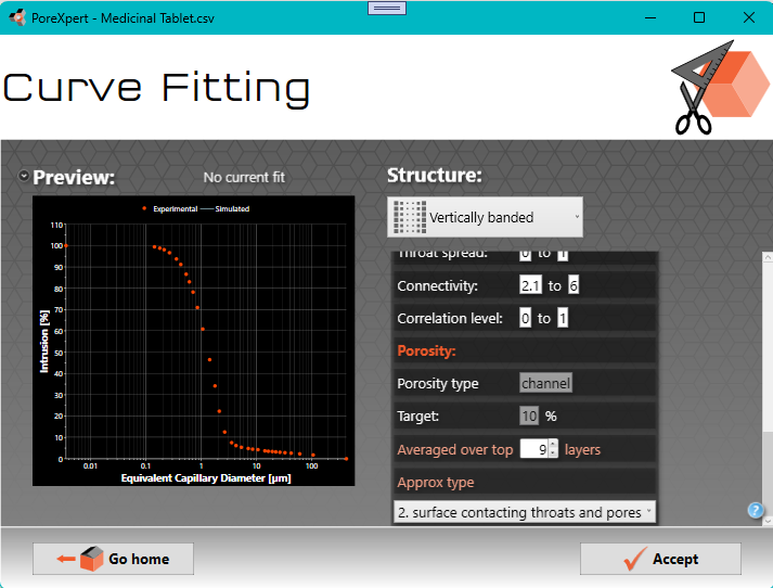
The screen shows you two defaults: Approx type 2, namely surface contacting throats and pores, and that the channel porosity is Averaged over top 9 layers. If the channel porosity is averaged over 4, 9 or 16 layers, then the effect can later be visualised as a 2x2. 3x3 or 4x4 grid surface (see Channel porosity visualisation).
With respect to the Approximation type, you need to consider what the image analysis of your electron micrograph is actually telling you about the porosity of the sample. The observed surface of a PoreXpert unit cell is always represented as the xy plane at maximum z, i.e. the top surface of the default unit cell image.
There are four options to choose from:
1. surface-contacting throats;
2. surface-contacting throats and pores (the default);
3. surface-contacting throats, pores and neighboring aligned throats;
4. all throats normal to the surface (i.e. in the -z direction relative to the observed (top) surface in the xy plane), and the pores of these throats.
All these approximations control how the PoreXpert unit cell represents your porous material. The appropriate level of approximation will depend on the smoothness of the surface viewed by electron microscopy (e.g. whether or not polished) and the nature of the material itself. The approximations relate to dimensions of the PoreXpert unit cell, not to the dimensions of your material - so you must judge how to map one onto the other. The following diagram helps to explain them further.

The four levels of approximation relating observation and image analysis of your micrograph to the PoreXpert unit cell
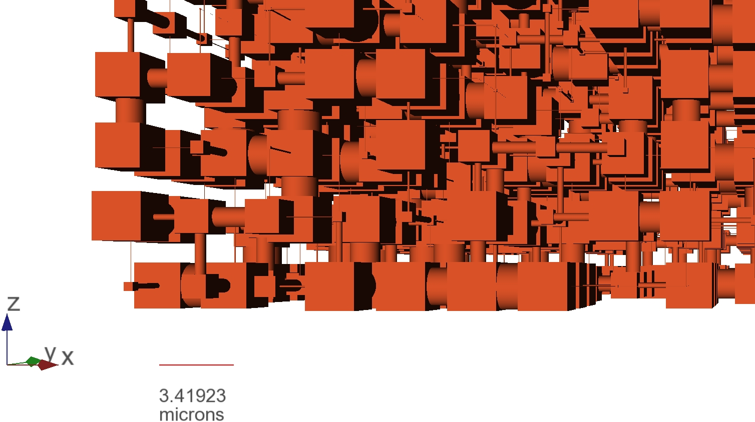
In order to make calculations tractable, the features within a PoreXpert unit cell are set on a Cartesian grid which is equally spaced on each Cartesian (x,y and z) direction. No pores can overlap, so the spacing between pores, i.e. the pore row spacing, is always larger than the largest pore that you model. In this example, the largest pore modelled is 2.37 μm. Once the unit cell is generated, the pore row spacing is shown by the small scale bar at the bottom left of the unit cell, and in this case we will find that it is 3.42 μm. So to choose the appropriate approximation, look at your electron micrograph, and map the pore row spacing onto it. Then ask yourself how far you are looking into the interior of the sample relative to that pore row spacing. The default is that you can see the surface throats (which are always visible), and the surface-connected pores behind them. Clearly when first choosing the approximation level, you have not yet generated a unit cell, so the choice is iterative - first use the default, generate the unit cell as exemplified below, look at the pore row spacing, and then reconsider whether the default approximation is the correct one.
The standard porosity is that based on pycnometry, or the porosity judged by mercury porosimetry, so is based on the entire accessible, or open, porosity. However, channel porosity is based on just the top surface of the unit cell. Normally, however, that is an unrepresentatively small part of the unit cell, especially for smaller unit cells such as the default 15 x 15 x15 array. So the channel porosity is calculated as an average over more than just the surface layer. The default is the top 9 layers. It is important to consider whether 9 layers gives a representation of the porosity of the whole unit cell. If, for example, a horizontally banded structure type is being used on a 15 x 15 x 15 grid, then 9 layers would not give a representative sampling of the whole structure. However, for the default vertically banded structure, 9 layers from 15 is a reasonable representation, as the layers do not fundamentally vary in the -z direction. The number of layers can be varied up to the maximum number of layers within the unit cell, but for visualisation purposes, it must be the square of an integer - i.e. 1, 4 9, 16 or 25, as will be explained.
Beware of choosing approximation 1 unless you have a perfectly smooth surface which genuinely only shows the emerging surface throats, such that you do not have any additional information to supply. Approximation 1 gives very little information to the simplex, and so its answers for different stochastic generations, unit cell sizes and number of layers for the porosity averaging will vary widely, to the extent that there may be no indication of the correct open porosity, and hence of other properties such as permeability. As you choose higher approximation type numbers, larger cell sizes, and larger number of layers over which to average the porosity, then simplex results for the different stochastic generations and unit cell sizes will converge much more closely onto what PoreXpert calculates as the correct open porosity. Whatever approximation type and number of averaging layers you choose, it is essential to compare different stochastic generations to check that you have a stably convergent answer.
You may then ask why approximation 1 is allowed. This is the closest approximation to porometry, but at the time of writing of this Help edition, we have not tried it on actual porometry samples.
If you understand how to generate the unit cell and find the pore row spacing, then you can now proceed to the Channel Porosity Visualisation page.
If not, then you can work through the detail in the Simplex Fitting page, or follow the summary screenshots below which guide you through how to do that for the current calcium carbonate (HydroCarb 60) example.
The fit for the calcium carbonate is as shown, with some of the fitting parameters displayed, including the largest pore size modelled (2.37 μm).

The operations list screen is as shown:
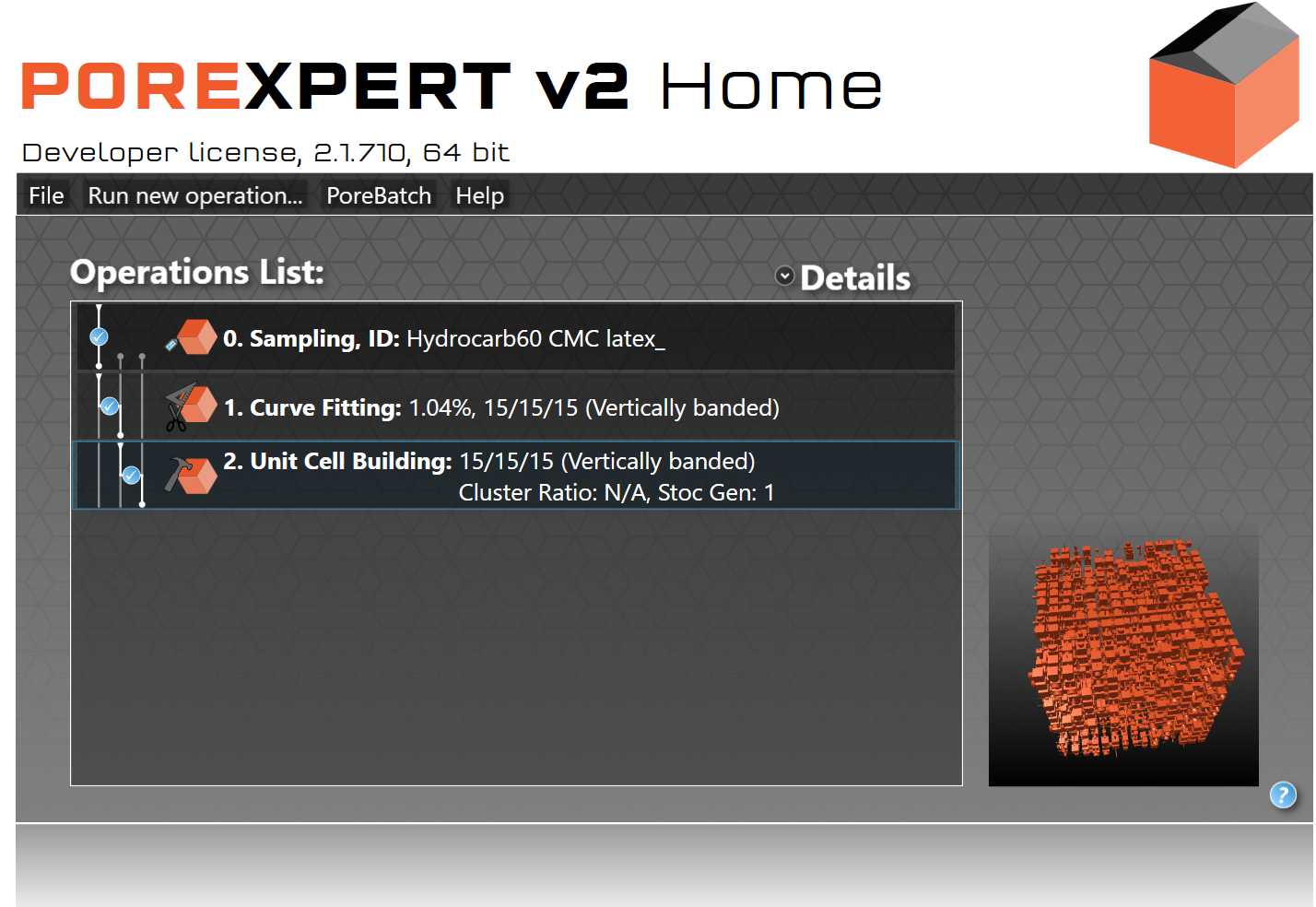
Left-clicking on operation 2. Unit Cell Building gives the choice of View mode:
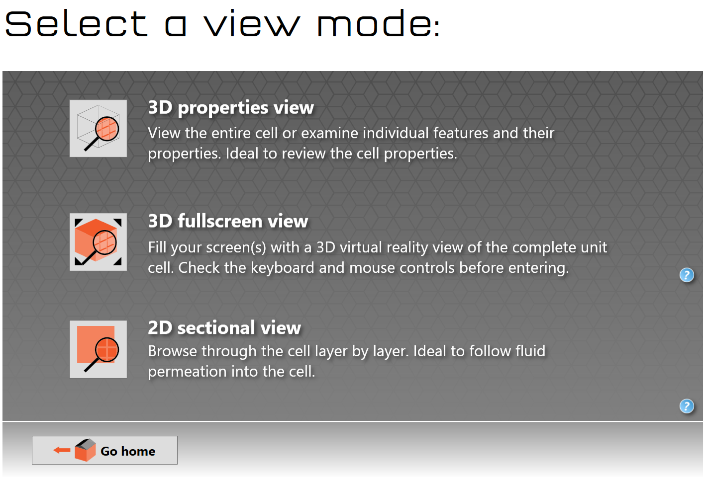
Left-clicking once on 3D fullscreen view displays the unit cell. Zooming in to the scale bar using the mouse controls shows the scale bar equal to the pore row spacing of 3.42 μm.
Now you can proceed to the Channel Porosity Visualisation page.